Storytelling – Kaggle Titanic Competition

As I told you in the first post I’d like to do some Competitions as my level increased. Now is time to start my Kaggle Competitions. Titanic, Machine Learning from disaster is one of the most helpful Competitions to start learning about Data Science. In this Kaggle page you will find a lot of help and you can learn how to start with different kind of languages Python, Excel and R, well in this blog I will do some Storytelling using R, concretely with Random Forest and Boosting. In near future I will post in comments or other posts more algorithms like Neural Network or SVM to solve this or other Competitions. But, what we know about the Titanic Disaster? 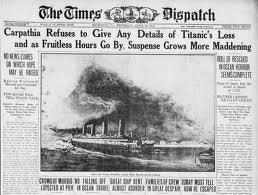A century has sailed by since the luxury steamship RMS Titanic met its catastrophic end in the North Atlantic, plunging two miles to the ocean floor after sideswiping an iceberg during its maiden voyage. Rather than the intended Port of New York, a deep-sea grave became the pride of the White Star Line’s final destination in the early hours of April 15, 1912. More than 1,500 people lost their lives in the disaster. In the decades since her demise, Titanic has inspired countless books and several notable films while continuing to make headlines, particularly since the 1985 discovery of her resting place off the coast of Newfoundland. Meanwhile, her story has entered the public consciousness as a powerful cautionary tale about the perils of human hubris. And what we know about this giant ship, Titanic had a length of 882 feet long and a weight of 46.000 tons, 9 decks and heigth about 175 feet. On board 2.224 passengers and crew (3.500), but lifeboats for only 1.178 people, incredible! 20 boilers & 162 furnaces burned thrugh 650 tons of coal per day, cranking out 16.000 horsepower. Top speed 24 knots, 4 smokestacks each 22 feet wide and 6 stories high. 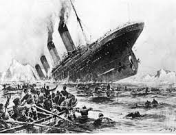It tooks 3.000 people over 3 years to build Titanic. In 1912 first class ticket 4.300 dollars and thirs class ticket 36 dollars.Titanic was cruising at 22 knots when it hit an iceberg on april 14, 1912 at 11:40 PM.The iceberg cut a hole into the hull between 220 and 250, finally, Titanic sank in less than 3 hours.The survival rate: first class 60%, second class 42%, third class 25% and Crew less than 25%. Titanic’s final resting place 350 miles southeast of newfoundland, Canada, 2.3 miles below the ocean’s surface. Turning back to reality and our Competition, we have Data for Training and Testing, we have a description about the variables:

VARIABLE DESCRIPTIONS:
survival        Survival
                (0 = No; 1 = Yes)
pclass          Passenger Class
                (1 = 1st; 2 = 2nd; 3 = 3rd)
name            Name
sex             Sex
age             Age
sibsp           Number of Siblings/Spouses Aboard
parch           Number of Parents/Children Aboard
ticket          Ticket Number
fare            Passenger Fare
cabin           Cabin
embarked        Port of Embarkation
                (C = Cherbourg; Q = Queenstown; S = Southampton)

Now take a look and listen what the Data tell us, first training data set:

str(train)
'data.frame':	891 obs. of  12 variables:
 $ PassengerId: int  1 2 3 4 5 6 7 8 9 10 ...
 $ Survived   : int  0 1 1 1 0 0 0 0 1 1 ...
 $ Pclass     : int  3 1 3 1 3 3 1 3 3 2 ...
 $ Name       : Factor w/ 891 levels "Abbing, Mr. Anthony",..: 109 191 358 277 16 559 520 629 417 581 ...
 $ Sex        : Factor w/ 2 levels "female","male": 2 1 1 1 2 2 2 2 1 1 ...
 $ Age        : num  22 38 26 35 35 NA 54 2 27 14 ...
 $ SibSp      : int  1 1 0 1 0 0 0 3 0 1 ...
 $ Parch      : int  0 0 0 0 0 0 0 1 2 0 ...
 $ Ticket     : Factor w/ 681 levels "110152","110413",..: 524 597 670 50 473 276 86 396 345 133 ...
 $ Fare       : num  7.25 71.28 7.92 53.1 8.05 ...
 $ Cabin      : Factor w/ 148 levels "","A10","A14",..: 1 83 1 57 1 1 131 1 1 1 ...
 $ Embarked   : Factor w/ 4 levels "","C","Q","S": 4 2 4 4 4 3 4 4 4 2 ...

str(test)
'data.frame':	418 obs. of  11 variables:

I love the package Amelia and how can we see the miss Data of our information: 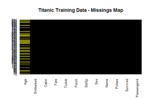We can see that we have around 20% of the ages missing.

summary(train$Age)
   Min. 1st Qu.  Median    Mean 3rd Qu.    Max.    NA's 
   0.42   20.12   28.00   29.70   38.00   80.00     177

About of our test Data we can see more or less the same.

summary(test$Age)
   Min. 1st Qu.  Median    Mean 3rd Qu.    Max.    NA's 
   0.17   21.00   27.00   30.27   39.00   76.00      86

In this case it’s important that you fill the NA’s values to have a better fit in your model, you can do it with several methods, for example:Replacing the missings with the average of the available values, in this case 29.70. Or you can do something more advanced like predicting the Age with the rpart algorithm:

summary(train$Age)
 modelage +                 data=train[!is.na(train$Age),], method="anova")
 train$Age[is.na(train$Age)] 

Another interesting way to see the Data and the correlation of the variables is using the corrgram package: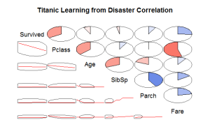We can see interesting information like the Fare variable it’s very correlated with the Pclass, then you can imagine the location of the passengers with this fare variable. Also another clear relation is that the variable PClass and Survived rate are very related, we can imagine that the people with higher class had more possibilities to survive. It’s curious that the Age variable is not much related with the Survived variable cause the child and women are the first in leave Titanic.

prop.table(table(train$Survived))

        0         1 
0.6161616 0.3838384

38% of people Survived and if we take a look the survival rate with PClass:

prop.table(table(train$Survived,train$Pclass))
   
             1          2          3
  0 0.08978676 0.10886644 0.41750842
  1 0.15263749 0.09764310 0.13355780

A 41% of third class died, third class was the 55% of the passangers, and 15% of first class survived.Well you can see inside the Data a lot of information and if you try to understand the situation you will imagine yourself living the tragedy and trying to understand what happened.Take a look inside the Trevor or Wehrley posts helps to see more deep understanding about the Data and the predictions. In this post I will show you the analysis of two important Algorithms Random Forest and Boosting.First of all you can find a good understanding in the Introduction to Statistical Learning with Application in R book, it’s free and you have the theoretical explanation and R examples to better understand how it works. In the Titanic Competition if you take a look in the forum lot of people try to solve it with RF.Random forests provide an improvement over bagged trees by way of a small tweak that decorrelates the trees. This reduces the variance when we average the trees. We build a number of decision trees on bootstrapped training samples. But when building these decision trees, each time a split in a tree is considered, a random selection of m predictors ischosen as split candidates from the full set of p predictors. The split is allowed to use only one of those m predictors. A fresh selection of m predictors is taken at each split, and typically we choose m pp | that is, the number of predictors considered at each split is approximately equal to the square root of the total number of predictors. If we try this algorithm with our Data:

set.seed(415)
 fit +                     data=train, importance=TRUE, ntree=2000)
# Variable importance
varImpPlot(fit)

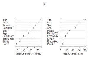We can see the importance of the Tittle variable, I have done a Tittle variable with the name for knowing the tittle of the people which is significant.I just try the algorithm RF with the best approach of trees, if you increase the number of trees the model doesn’t improve the results.

> Prediction > submit > write.csv(submit, file = "2000treeforest.csv", row.names = FALSE)

If you’ll do a submission of this Prediction you obtain a 0.77512 that’s give you a 1200 position from 1855 competitors.

set.seed(415)
fit +                data = train, controls=cforest_unbiased(ntree=2000, mtry=3))
Prediction submit write.csv(submit, file = "2000treesmtry3forest.csv", row.names = FALSE)

If we make a submission we obtain 0.81340, until the 72 position (well you have people with this result until 200 more or less). This implementation of the random forest (and bagging) algorithm differs from the reference implementation in randomForest with respect to the base learners used and the aggregation scheme applied. Conditional inference trees, see ctree, are fitted to each of the ntree perturbed samples of the learning sample. Most of the hyper parameters in ctree_control regulate the construction of the conditional inference trees. Hyper parameters you might want to change are: 1. The number of randomly preselected variables mtry, which is fixed to the square root of the number of input variables. 2. The number of trees ntree. Use more trees if you have more variables. 3. The depth of the trees, regulated by mincriterion. Usually unstopped and unpruned trees are used in random forests. To grow large trees, set mincriterion to a small value. The aggregation scheme works by averaging observation weights extracted from each of the ntree trees and NOT by averaging predictions directly as in randomForest. See Hothorn et al. (2004) and Meinshausen (2006) for a description. Predictions can be computed using predict. For observations with zero weights, predictions are computed from the fitted tree when newdata = NULL. Ensembles of conditional inference trees have not yet been extensively tested, so this routine is meant for the expert user only and its current state is rather experimental. However, there are some things available in cforest that can’t be done with randomForest, for example fitting forests to censored response variables (see Hothorn et al., 2004, 2006a) or to multivariate and ordered responses. Using the rich partykit infrastructure allows additional functionality in cforest, such as parallel tree growing and probabilistic forecasting (for example via quantile regression forests). Also plotting of single trees from a forest is much easier now. Unlike cforest, cforest is entirely written in R which makes customisation much easier at the price of longer computing times. However, trees can be grown in parallel with this R only implemention which renders speed less of an issue. Note that the default values are different from those used in package party, most importantly the default for mtry is now data-dependent. predict(, type = "node") replaces the where function and predict(, type = "prob") the treeresponse function. Moreover, when predictors vary in their scale of measurement of number of categories, variable selection and computation of variable importance is biased in favor of variables with many potential cutpoints in randomForest, while in cforest unbiased trees and an adequate resampling scheme are used by default. I have to make some improvements with this RF algorithm to better fit the model, I will do some testing and I’ll inform you about the results. Let’s take a look about boosting, like bagging, boosting is a general approach that can be applied to many statistical learning methods for regression or classication. We only discuss boosting for decision trees. Recall that bagging involves creating multiple copies of the original training data set using the bootstrap, setting a separate decision tree to each copy, and then combining all of the trees in order to create a single predictive model. Notably, each tree is built on a bootstrap data set,independent of the other trees. Boosting works in a similar way, except that the trees are grown sequentially: each tree is grown using information from previously grown trees.

Grid +   n.trees = c(2000),
+   interaction.depth = c(10) ,
+   shrinkage = 0.001)
> 
> # Define the parameters for cross validation
> fitControl 
>
> # Initialize randomization seed
> set.seed(1805)  
> GBMmodel +                   data = train,
+                   method = "gbm",
+                   trControl = fitControl,
+                   verbose = TRUE,
+                   tuneGrid = Grid,
+                   metric = "ROC")

The most interesting parameters are:

Grid +   n.trees = c(2000),
+   interaction.depth = c(10) ,
+   shrinkage = 0.001)

you have to test the best approach for each parameters.If we check the results with the training data:

> GBMpredTest = predict(GBMmodel, newdata = train)
> confusionMatrix(GBMpredTest, train$Survived)
Confusion Matrix and Statistics

          Reference
Prediction   0   1
         0 518  81
         1  31 261
                                          
               Accuracy : 0.8743          
                 95% CI : (0.8507, 0.8954)
    No Information Rate : 0.6162          
    P-Value [Acc > NIR] : < 2.2e-16       
                                          
                  Kappa : 0.7267          
 Mcnemar's Test P-Value : 3.656e-06       
                                          
            Sensitivity : 0.9435          
            Specificity : 0.7632          
         Pos Pred Value : 0.8648          
         Neg Pred Value : 0.8938          
             Prevalence : 0.6162          
         Detection Rate : 0.5814          
   Detection Prevalence : 0.6723          
      Balanced Accuracy : 0.8533          
                                          
       'Positive' Class : 0

We have an accuracy of 87% and a very good rate for the other parameters.If we do the submission we obtain a result 0.81818, a little bit better than RF, you obtain a position of 35 to 71 (with the same result).But what happens if you put a better shrinkage parameter 0.1, this are the results:

> GBMpredTest = predict(GBMmodel, newdata = train)
> confusionMatrix(GBMpredTest, train$Survived)
Confusion Matrix and Statistics

          Reference
Prediction   0   1
         0 543   8
         1   6 334
                                          
               Accuracy : 0.9843          
                 95% CI : (0.9738, 0.9914)
    No Information Rate : 0.6162          
    P-Value [Acc > NIR] : 
An incredible accuracy, more than 98.4%. and the rest of parameters are close to 1, then we can conclude that the model fits almost perfectly the Training Data model, but what happens with the Test Data if we do a submit with this model the result is 0.71770, but how it's possible? well this is an example of over fitting, yes the model is perfect for the Training Data but the Test Data it's a little bit different then, with this prediction we obtain a worst result. Now the challenge here is to try to understand how to obtain a 1 prediction, maybe the difference is cleaning or adapting the data to the story in a better way or maybe I have to test with some improvement in the training parameters to better fit the model.At this moment we can observe the potential of Data Science but this is only the top of the iceberg.

---